We were tasked to enhance an image by changing the cummulative distribution function (CDF) of an image. The CDF of a graylevel is just the sum of all the number of pixels with the grayvalue, from grayvalue of 0 to some grayvalue K. This is normalized by the number of pixels present in the image. The CDF is obtained by obtaining the histogram of the grayscale of an image. The histogram is then normalized to obtain the probability density function of the image (PDF). Obtaining the cummulative sum will give us the CDF. The figure we enhance in this activity is shown in figure 1, along with the CDF of the image.
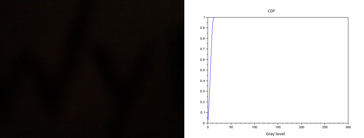
Figure 1. The image to be enhanced is on the left and the Cummulative Distribution Function is on the right. The CDF shows a sudden increase in the amount of pixels having low gray levels. This means that the picture is mostly black.
LINEAR
First, to enhance the image in Figure 1, we impose a linear CDF, that is, a normal PDF. This is quite easy to do since the goal is a linear CDF, we just need to multiply the CDF of the original image by 255. The general process is shown in figure 2.
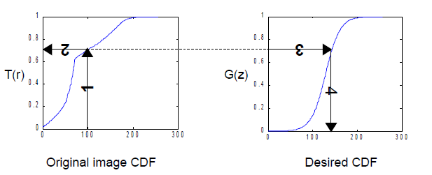
Figure 2. The steps on how to alter the gray scale distribution. (1) The gray level of the pixel must be known, and the corresponding value in the CDF. Then the CDF value is projected onto the desired CDF, and finally, the corresponding gray level of the pixel is the new gray level.[1]
For the first part, we obtain the enhanced image with a linear desired CDF. Figure 3 shows the enhanced image, along with the CDF of the resultant image, and the desired CDF.
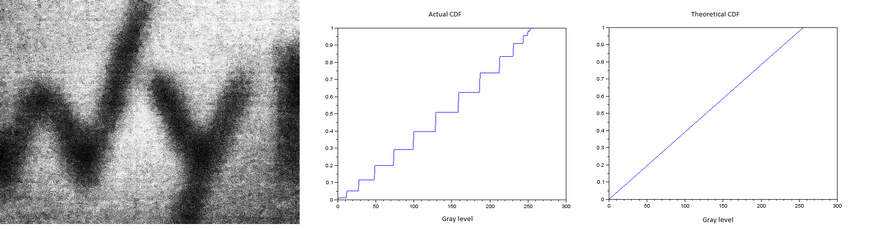
f igure 3. The enhanced image with the resulting CDF(center) and the desired(right) CDF. It can be seen that though the resulting CDf kinda follows the desired CDF, the resulting CDF shows a ladder pattern
From figure 3, it can be seen that the resulting CDF follows the desired CDF but has a ladder pattern. This means that even though we force the CDF to change, the previous CDF of the image still acts as a constraint, preventing the resulting CDF to completely follow the desired CDF.
SIGMOID
A sigmoid function is a function that looks like the letter S. The function is given by:
S(t) = 1/(exp(-t) + 1) (1)
If we add the scaling factors, the translation and the size of the sigmoid function can be changed. Applying the scaling factors, (1) becomes:
S(t) = 1/(exp((-t + T)/d) + 1) (2)
Where T is the translation and d is the width of the sigmoid. Conversely, we can find the t if we are given the S(t). In our case, the S(t) is the desired CDF and t is the gray level corresponding to the CDF. Doing some mathematical derivation, we arrive at:
t = -dlog(1/s – 1) +T (3)
First we need to find the optimum T. Our code (see below), has a line with a function uint8. this ensures that the values are between 0 and 255. This function obtains the modulo of every value of 256. Choosing a random d to find the optimum T, (d = 32), we generate the following images, with different T.
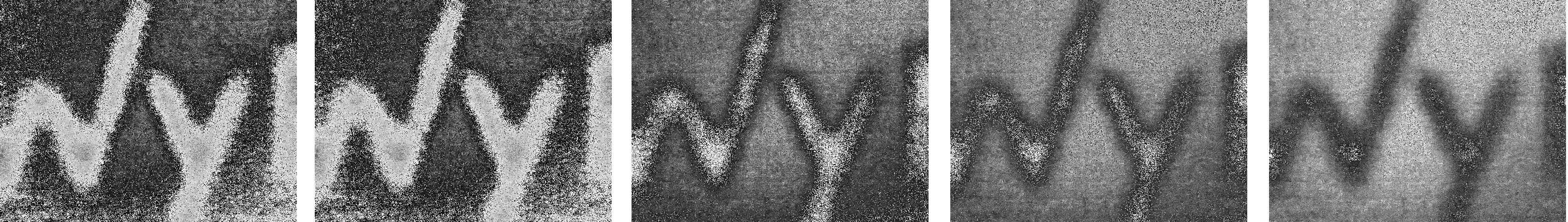
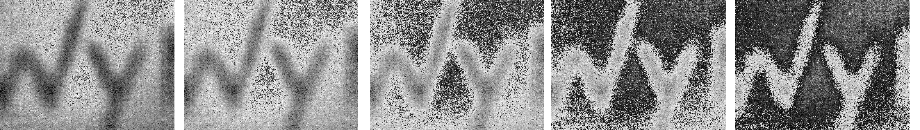
Figure 4. Images showing different translation T in the computation. On the upper left is T = 0, and with 30 increments thereafter. We know that the image was created with a black pen on a white background. In the figure above, the image we picked is the image in the lower leftmost figure. this is because, the contrast is not that high or low.
From figure 4, we used T = 150. For the next part, we change the width factor d in the calculation, from 1, 2, 4, 8, 16, 32, 64, and 128. Figure 5 shows the CDF from 1 – 128 (in exponents of 2). (I call it width since it seems to be similar to the gaussian standard dev where beam width is 1/e)
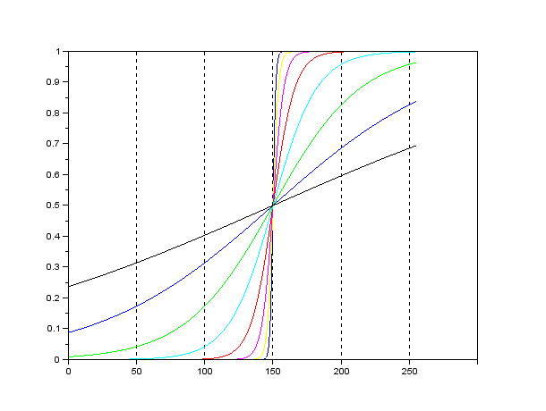
Figure 5. The CDF used, with different CDF sizes ( innermost is 1 while outermost is 128, in exponents of 2)
Using the CDFs above as the desired images, we generate the following images(with the corresponding resulting CDF’s):

Figure 6. The enhanced images with different CDF widths. Left column has width = 1, 2, 4, 8(top to bottom), While the right column has width = 16, 32, 64, 128 (top to bottom)
What seems peculiar in figure 6 is that, when the CDF width is chosen to be 128, there can be no discernible letter in the image. Looking at the image, we could say that the most enhanced image would be the image with width equal to 32 and translation equal to 150. it can be seen that the resulting CDF follows the desired CDF exept for the lower 3 images in the right column.
Other softwares also have this kind of manipulation. The histogram can be manipulated by dragging the diagonal line. however I am not going to discuss that here.
I give myself a credit of 11/10 since i investigated the effect of translating and manipulating the width of the sigmoid.
[1] Laboratory manual by Dr. Maricor Soriano
CODE for Sigmoidim = imread(‘C:\Users\ledy_rheill\Google Drive\Documents\Academics\13-14_1stsem\AP186\activity 6 27 Jun 2013\image.png’);
im_gray = rgb2gray(im);//convert to grayscale
his_plot = CreateHistogram(im_gray, 256); // obtain histogram
size_xy = size(im_gray);//obtain sizes for normalizatio
narea = size_xy(1,2) * size_xy(1,1); //take area for normalization
summed_his = cumsum(his_plot)/area; //normalized cummulative sum
//first we use a linear cummulative distribution function where the probability distribution function is normal (cdf is a line), therefore we just multiply the cdf of the original image by 256
new_summed = summed_his(im_gray + 1);//converts the image gray values to the corresponding cummulative sum. there are 256 values of cdf, but array starts at 1
im_gray2 =-1*log(2 ./(new_summed + 1.000002) – 1) ;// since CDF is linear, the correspondence is also linear, so we just multiply the CDF by the value of the pixel with cdf equal to 1, which is
max(new_summed) * 256 -1im_gray_new2 = matrix(real(im_gray2), size_xy(1,1), size_xy(1,2));// since it was flattened to one d, we convert it back to 3D
im2 = uint8(im_gray_new2);//convert to 8bit imageimshow(im2);
his_plot2 = CreateHistogram(im2);summed_his2 = cumsum(his_plot2)/area
imwrite(im2, ‘C:\Users\ledy_rheill\Google Drive\Documents\Academics\13-14_1stsem\AP186\activity 6 27 Jun 2013\sigmoid_cdf_128width_flower.png’)
