In the old age where a diskette (ha! hipsters can relate) is equivalent to today’s USB in terms of usefulness, Storage was once a problem, and in finding a way to solve this, they have come across what is currently known as image compression, which is still being used today (hello JPEG). In this activity, we show how to compress images using Principal Components Analysis (PCA).
Basically what PCA does is that it converts a set of correlated signals into orthogonal functions whose sums (with their respective coefficients) can reconstruct any of the signals. (I do not want to indulge in here. :PPP) If we have a set of functions, f1, f2, f3, …. , fn, then we can obtain a set of orthogonal functions W1, W2, W3… Wm such that:
Where 


![[lambda, facpr, comprinc] = pca(X);](https://s0.wp.com/latex.php?latex=%5Blambda%2C+facpr%2C+comprinc%5D+%3D+pca%28X%29%3B+&bg=eeeae8&fg=4a4a49&s=0&c=20201002)
where facpr is the matrix containing the principal components and comprinc the matrix containing the coefficients. Lambda gives the percent contribution of each principal components to the signals.
In image compression, what we do is that we cut our image into 


There will be 
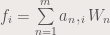
We use a picture of a cat (well its a tiger but…. still a cat).

A cat.
In the figure below, we show the difference of the original picture (in grayscale) to the reconstruction images.
The topleft figure is the grayscale image of the cat. The top center is for n=1, top right is for n = 5, bottom left is n = 10, bottom center is n = 50 and bottom right is n = 100.
From the figure above, we can see that the higher the number of principal components used, the better the quality. However, it can be observed that for n = 50 and n = 100, the images do not vary much. This is due to the percent contribution of the principal components.
In the next figure, we show what the principal components look like.

The principal components are each 10 x 10 part of this picture.
We show another example. This one came from the anime Fate zero, where the protagonist is a female swordsman…..well you can search it if you like.
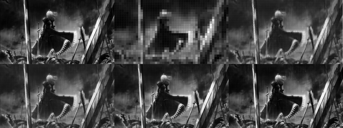
The number of principal components are the same as the cat figure.
The author gives himself a score of 9/10 for this work. He acknowledges Mr. Tingzon for the help. 🙂
Sources:
Wikipedia
Dr. Maricor Soriano
