We try to enhance images in the Frequency Domain (hello again, FFT. Haha). For some background, it is recommended to read on the Fourier transform first. 🙂
Anyways, Image enhancement is almost always done in the frequency domain. This is because noise and spurious parts of the image cannot be removed from the image itself. However, these unwanted distortions can be removed in the frequency domain since they have different (higher) frequencies than the important details of the image. What generally happens is we multiply a mask in the frequency domain to remove the higher frequencies. But if we multiply in the frequency domain, we are actually performing a convolution in the image domain. So before everything else, lets discuss convolution! (For a little bit of background, you may want to read on my previous post. Or search it on google. Or read arfken. Whichever.)
Convolution is actually smearing of two functions to create another function that has the properties the two functions. This is in contrast to correlation, where the resulting function is the similarity of the two functions. In more simplified words, convolution is a union of properties, while correlation is an intersection of properties. A convolution is presented below:

or:

The integral is quite cumbersome to work with, especially when coding. There are some programming languages that have a convolution function, but generally the integral itself has to be worked out. Thankfully, performing the Fourier transform simplifies things:

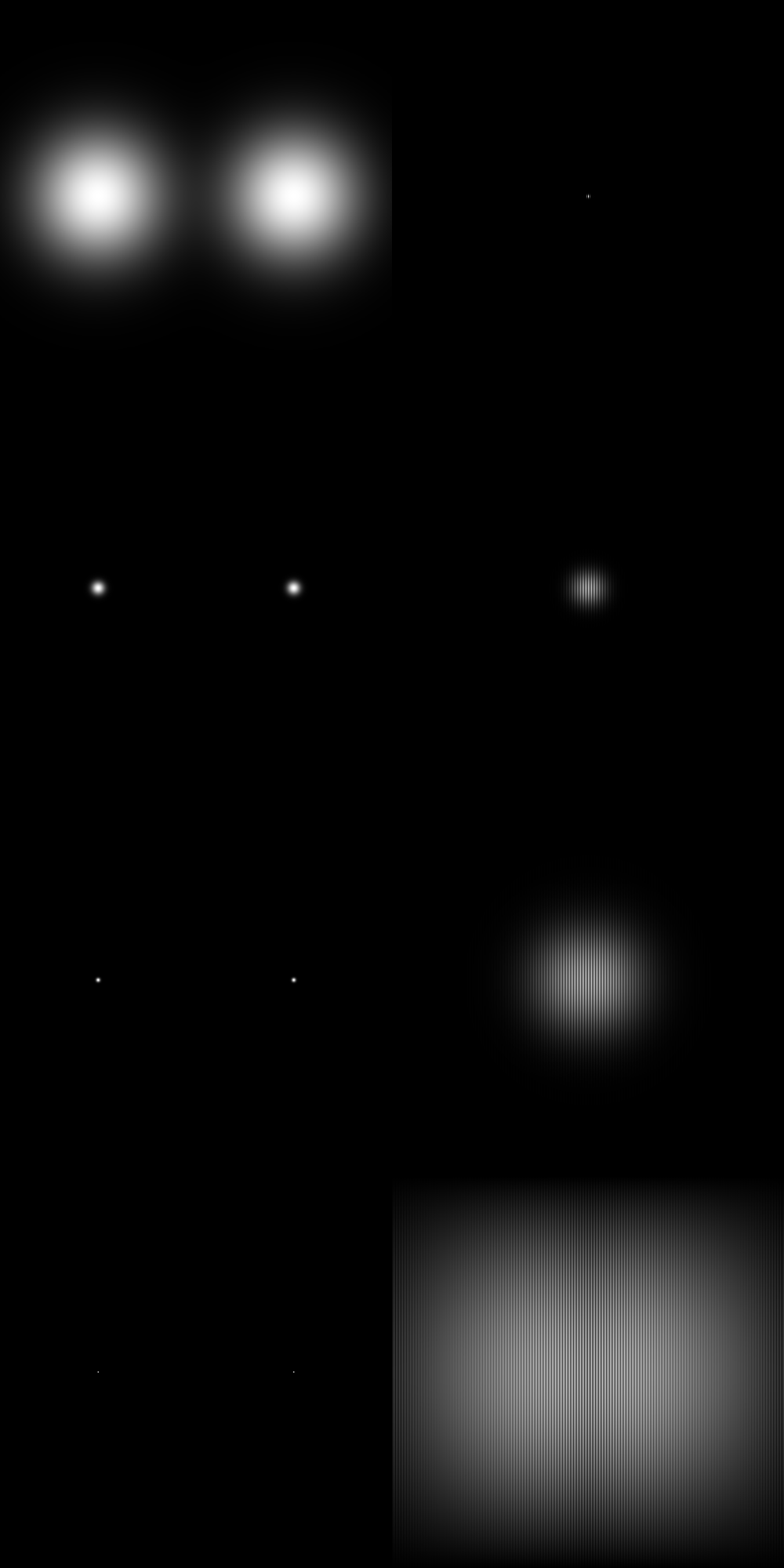
where the  is the Fourier transform operator. I have already performed some convolution myself. Figure 1. shows a the result of convolving circles of different sizes and their Fourier transforms.
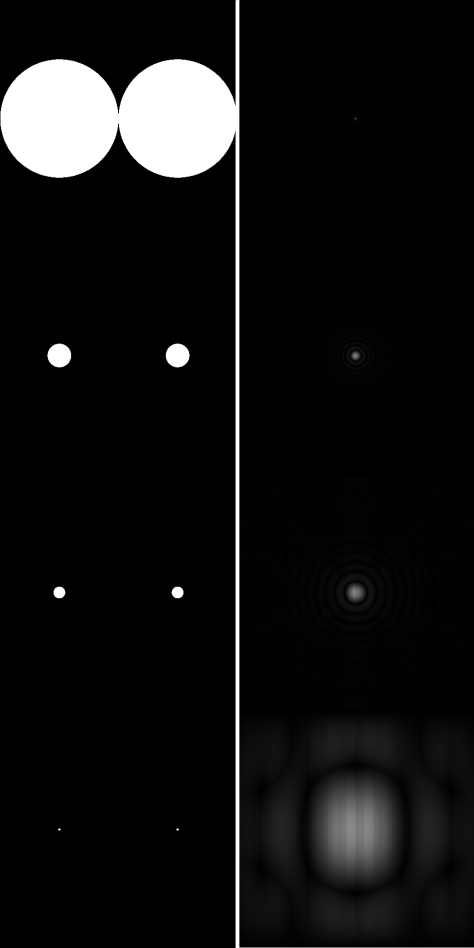
Figure 1. The left side shows the result of the convolution in the image domain. Convolving with a sum of Dirac delta functions is just placing the center of the image in that position. In the frequency domain, the convolution is just the multiplication of the Fourier transform of each function.
The Fourier transform of a two-Dirac delta function which is symmetric wrt the y-axis is a sinusoid while the Fourier transform of a circle is an Airy pattern. The airy pattern is very prominent in the right side, though the sinusoid is not that discernible. This could be due to the fact that the Dirac deltas are far from the center, hence they are high frequency. High frequency in images are the ones that cannot be discerned if the image is rescaled to a smaller size.
We show some more convolution. This time the same Dirac delta function and a square (figure 2), and a Gaussian (figure 3).
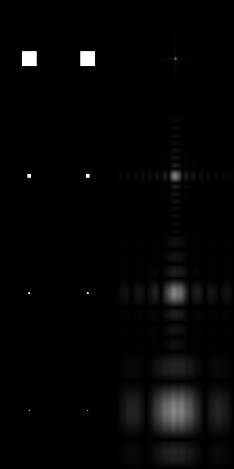 Figure 2. Convolution of a square and the Dirac delta function.
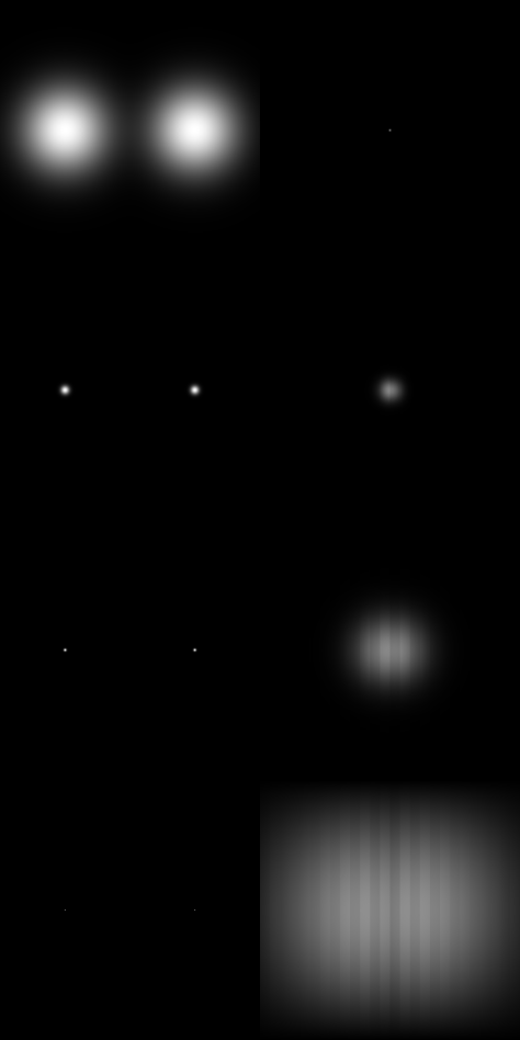
Figure 3. Convolving a gaussian with the same Dirac delta function.
The above images show the end result when the convolution is done in one plane; multiplication is done on the other. However, I haven’t really shown you what really happens when you convolve two things in the same plane. Figure 4 show what happens when you convolve two functions.
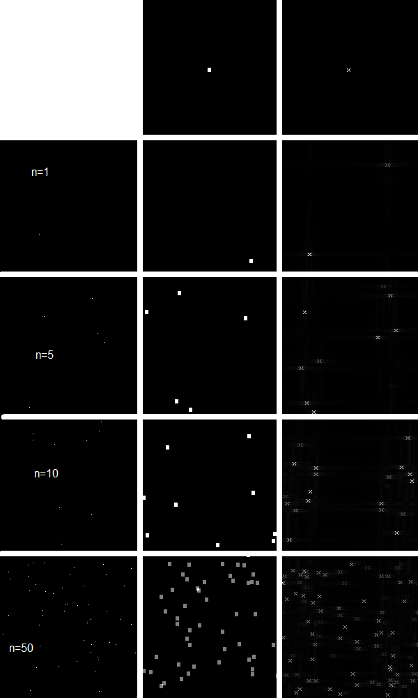
We generate Dirac deltas in random places and convolve them with the following patterns (Im sorry, i wasn’t able to convolve them with the same set of Dirac deltas. Since the position are random, the Dirac deltas are not the same. :[..)

Figure 4. n is the number of Dirac deltas. A comparison shows that for the x pattern, we can observe ghost spectra.
Figure 4 shows the convolution between Dirac deltas and square function, and Dirac deltas and the x pattern. The square and the x pattern is simply place where the Dirac delta is placed.
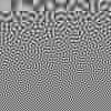
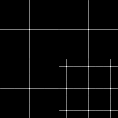
Figure 5 shows the Fourier transform of uniformly distributed Dirac deltas in the x and y axis, with different distances from each other.
 Figure 5. The FFT of Dirac deltas in the x and y-direction with different distances from each other (1, 2, 4, and 8).
Image enhancement
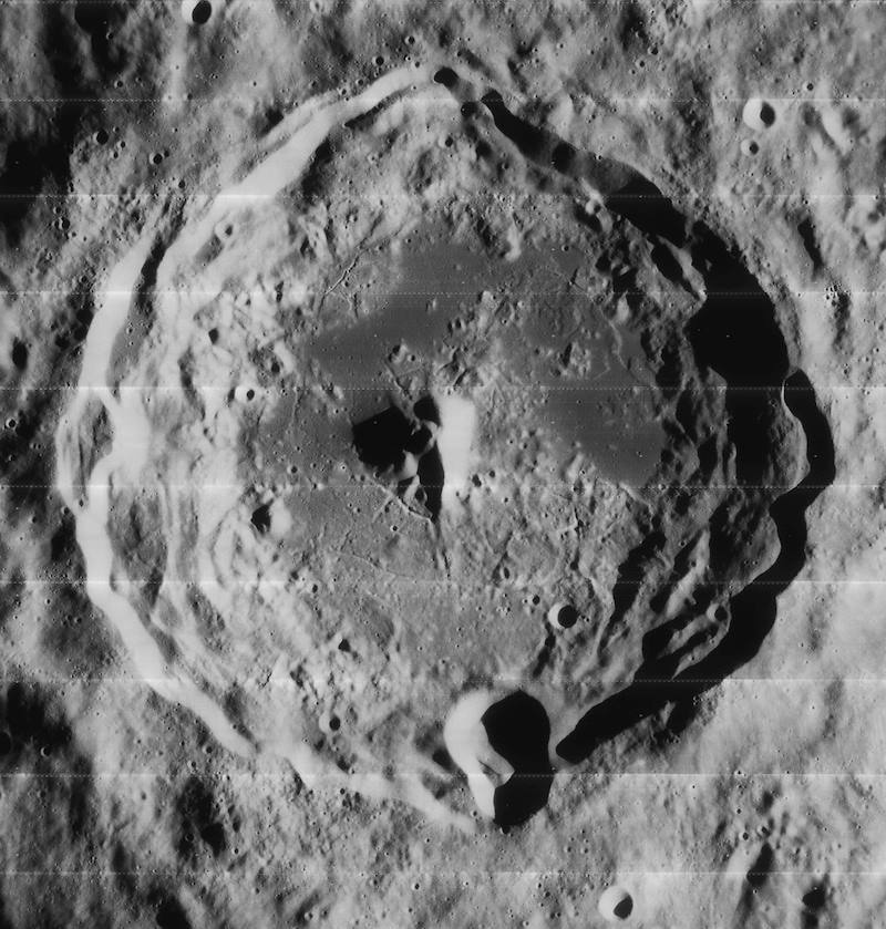
Now we finally get to enhance some image! First off, we’ll try to enhance the famous image, the image from the lunar orbiter, shown in figure 6.

Figure 6. The image from the lunar orbiter.
As observed, there are a lot of spurious white lines in the image. This is because the image was transmitted part by part so there was some irregularity. We try to remove the whitelines by multiplying a mask in the Fourier domain. Applying FFT:
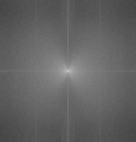
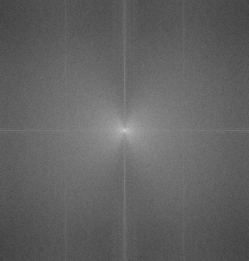
Figure 7. The image is in log scale since the low frequency details have higher magnitude such that all the other details seem black.
We can see a lot of white noise, though their magnitude is smaller. If we refer to figure 5, we can estimate the frequency of the inconspicuously white lines, and in figure 7, that would be the straightlines. We multiply a mask, an example of which is shown in the next figure.
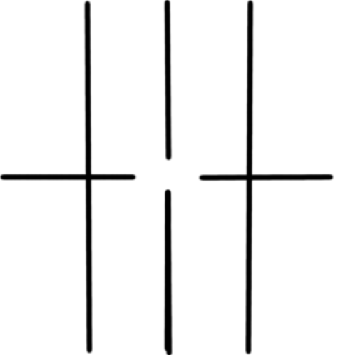
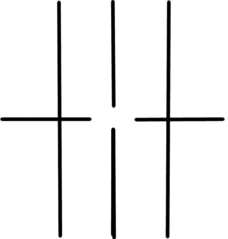
Figure 8. The mask that was used.
Observing figure 8, we may point out that the center is being left out. This is because, in many images, the important details often have low spatial frequency (of course this applies to most signals as well), so we have to retain those information. We multiply figure 8 and 7 then apply IFFT. The result is shown in figure 9.
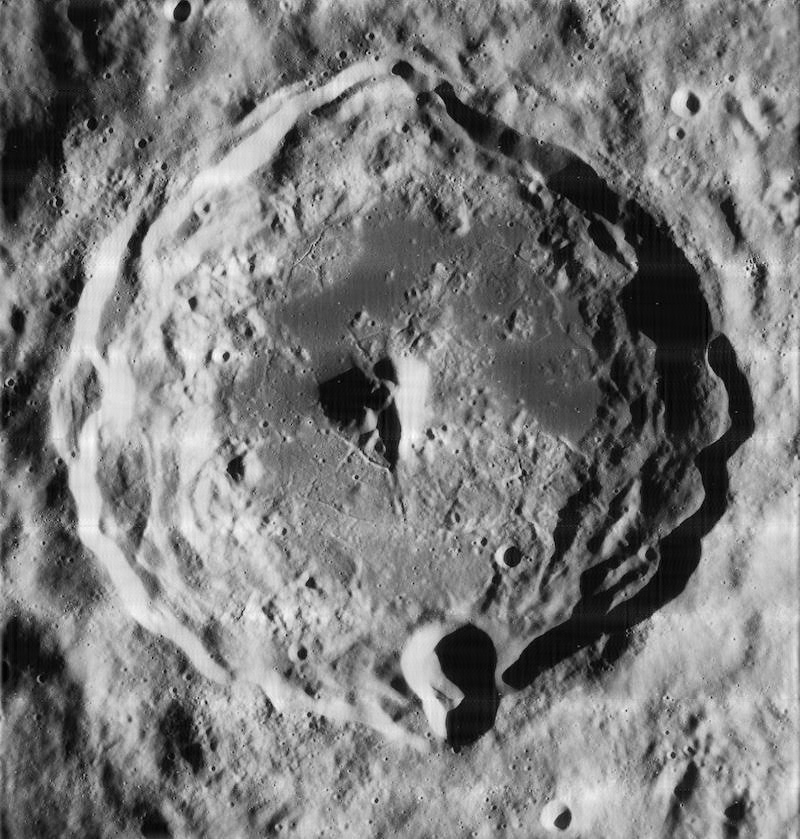
 Figure 9. The output of applying a mask in the Fourier domain.
In figure 9, the white lines become lesser. However, they can still be seen. It is recommended to thicken the lines in figure 8 to remove more. However, this has the probability of removing some important detail, so we did not do it here.
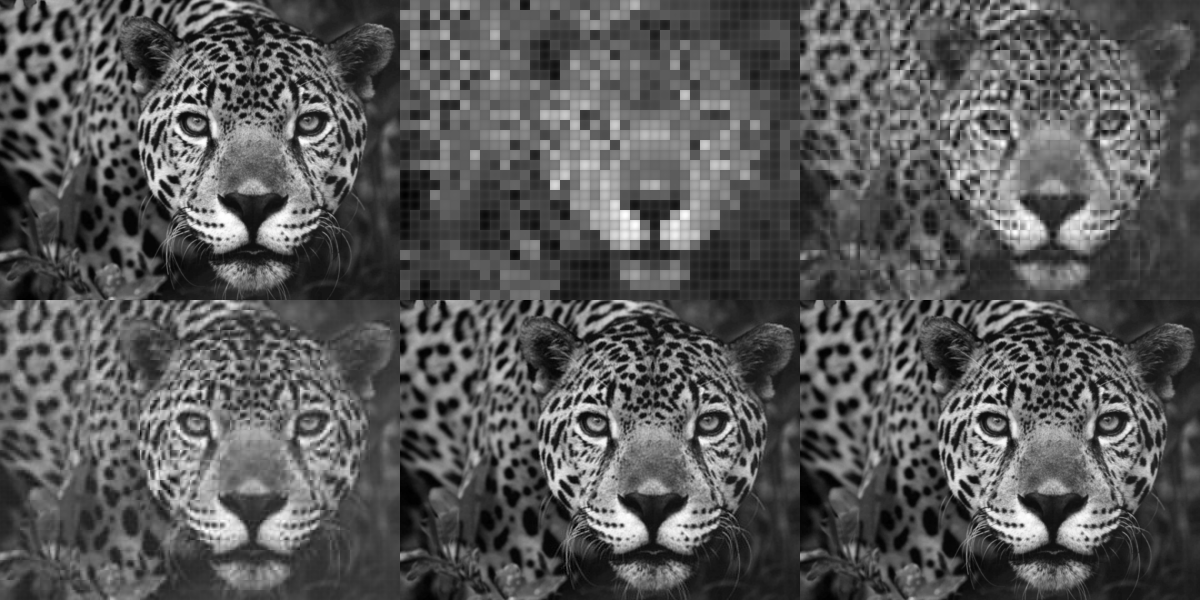
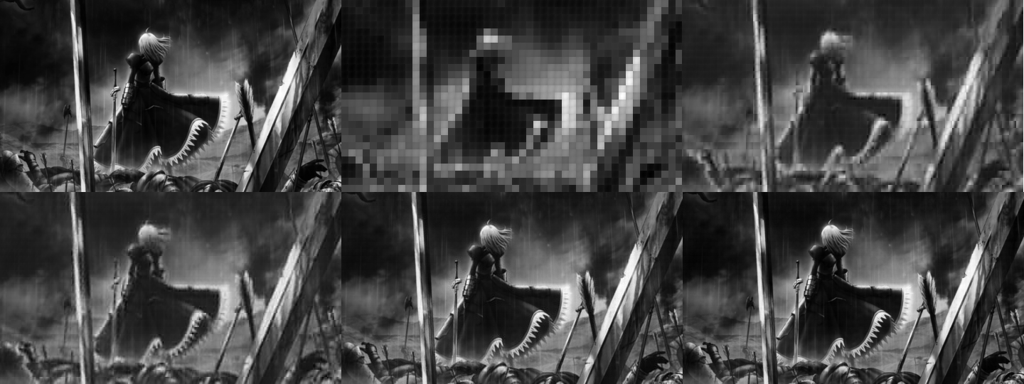
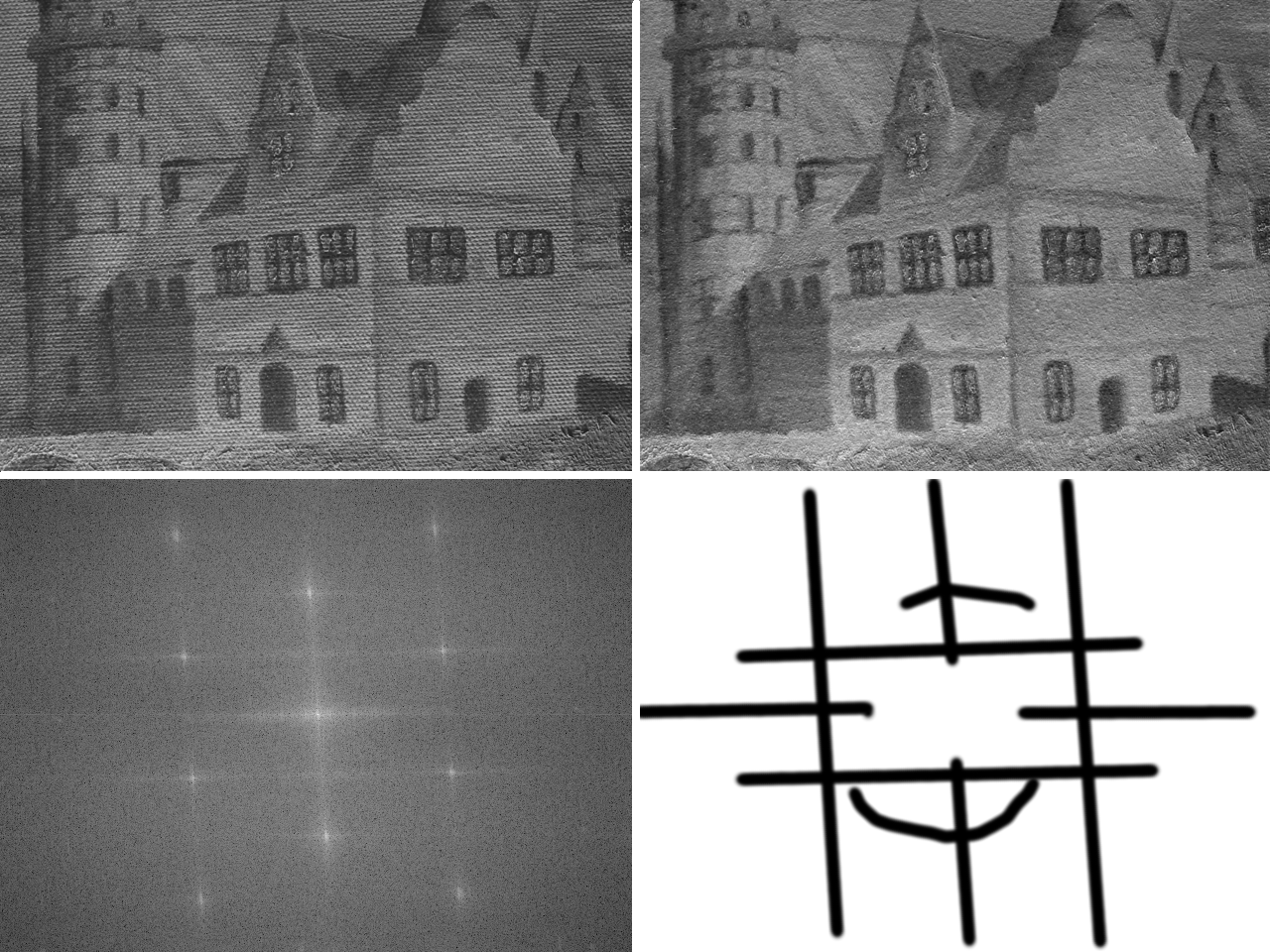
In figure 10, we show another example of an enhanced image, a painting by Dr. Vincent Daria, Fredericksborg.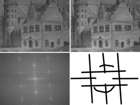
Figure 10. The Fredericksborg.
The top left image is the painting before doing anything (converted to grayscale). The lower left is the FFT then the lower right is the mask. After applying the mask to the FFT of the image and applying IFFT, the top right image is obtained. It is obviously cleaner than the one on the right. The brush strokes are removed.
The author gives himself 10/10 for completing the minimum requirements.
acknowledgements to Abby for helping.


![[lambda, facpr, comprinc] = pca(X);](https://s0.wp.com/latex.php?latex=%5Blambda%2C+facpr%2C+comprinc%5D+%3D+pca%28X%29%3B+&bg=eeeae8&fg=4a4a49&s=0&c=20201002)