Greens area

For this activity, we were tasked to obtain the area of shapes using greens theorem. using the edge function of scilab, we are to obtain the area and by analytically solving for the area, we are to compare the results from the greens theorem to the analytically solved area.

first, I obtained the area of 10 circles. The result of the edge function is also shown. (I only show one circle).

Figure: the circle on top, the result of the edge function on the bottom.

After obtaining the edge, I obtain the area using the discretized green’s function. I repeat the process for 10 different circles to obtain the average deviation from the answer using the equation for the area. I obtained a deviation of 0.62%.

I also did the same thing for rectangles.

Figure: Edge detection of a rectangle

After doing the same process for rectangles, I obtain a deviation of 0.46%.

We are also tasked to obtain the area of any location of interest using the greens theorem. I chose to find the area of the Quezon Memorial Circle, which has an area of 27 hectares, or 270,000 square meters. After isolating the Quezon Memorial Center and obtaining the edge, I have the following images:

After applying the Green’s theorem, i obtained an area of 233935.44 square pixels. Using the scale bar, 90 pixels is 100 meters, therefore 8100 square pixels is 10000 square meters. using ration and proportion, the area of the memorial center is 288809.1853 sq. m. or 28.88 hectares. This value is 7.0% from the theoretical value.

I obtained the area of the Quezon memorial center from:

http://www.1stphilippines.com/pc-30f6af23af986d2e822e18015fd22ce1.html

The author gives himself a grade of 9/10 since he was only able to do the rectangle and the circle.

Tinkering with images :)

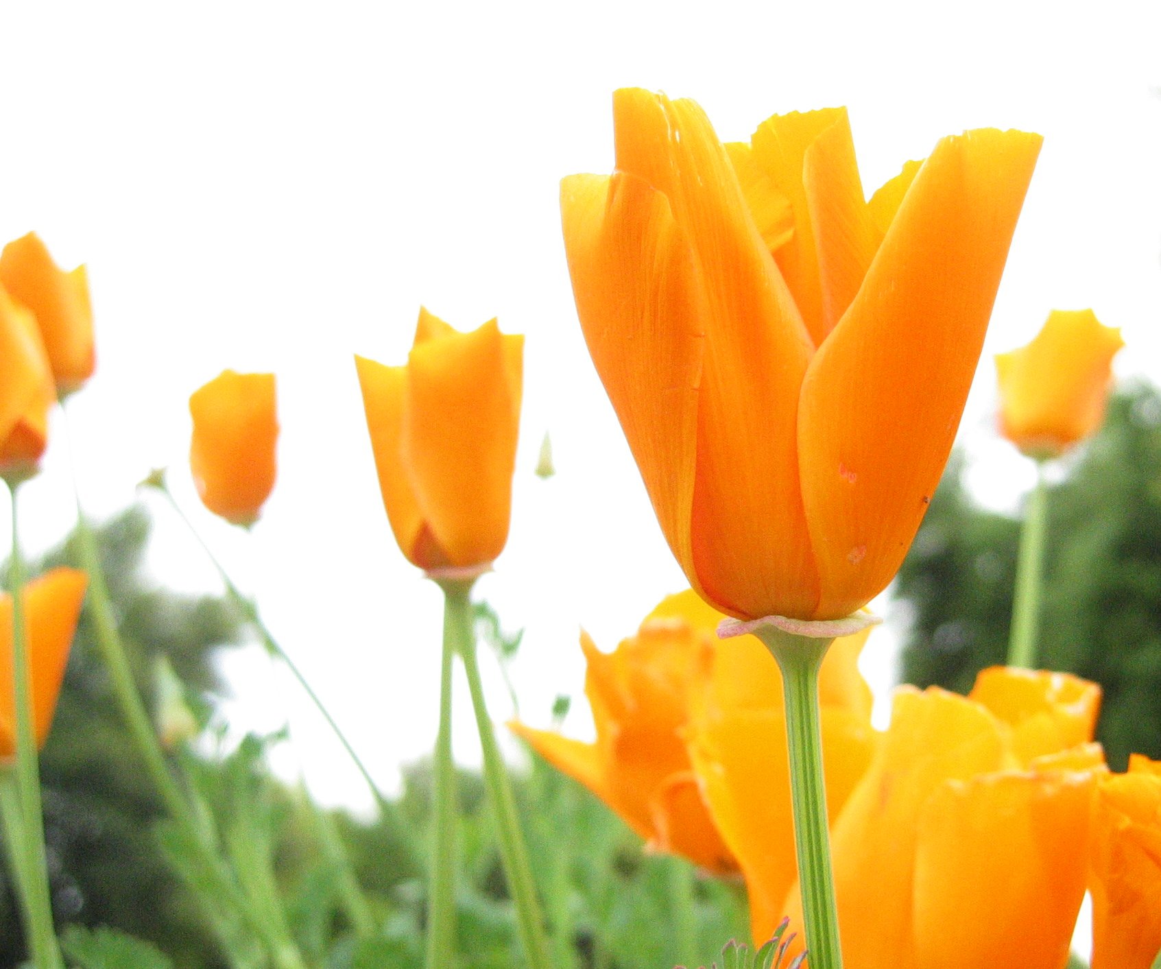
For this activity, we were told to tinker with images and their properties. first stop was to know properties of images downloaded from the web. And since i like flowers, let me show you some of them 🙂 (i’ll only show the camera or the software used)

Canon PowerShot S45,  1693 x 1413 pixels, 24-bit 180dpi resolution (vertical and horizontal)

F-stop : f/2.8, exposure: 1/1000 s, exposure bias: -2 step

focal length = 7mm, max aperture : 2.9685

no flash, auto white balance, no zoom, EXIF version 0220

279KB

(no camera information)

1920 x 1080 pixels, 24-bit, 96 dpi (vertical and horizontal)

focal length : 35mm

272KB

(no camera information) \

1920 x 1080 pixels, 24-bit, 96dpi (vertical and horizontal)

90.1KB

Canon PowerShot S2 IS,

1024 x 768 pixels, 24-bit, 72 dpi (vertical and horizontal)

compressed bits/pixel: 5

F-stop: f/4, exposure: 1/160 s, exposure bias: 0 step

focal length: 14mm, max aperture: 3.625

noflash, auto white balance

152KB

camera maker: OLYMPUS IMAGING CORP., model: FE310,X840,C530

1024 x 768 pixels, 314 dpi, 24-bit

f-stop : f/3.3, exposure: 1/30 s., ISO speeed: ISO – 180

exposure bias: 0-step, focal length: 6mm., max aperture: 2.97, metering mode: center weighted average, no flash

219 KB

Okay guys you might be confused at those details. let me explain them in a bit.

At the first lines, we show the manufacturer and the model of the camera used. We have canon and olympus. The next line shows the number of pixels or the size of the image itself. Then we have the dpi, or the dots per inch. This is the resolution of the camera. It basically shows how much dots does an inch contain. The higher the dpi, the higher the resolution of the camera, and also, the higher the image size on drive. 🙂 As a proof of that, let’s look at images 4 and 5 because they have the same size. Image 5 has dpi of 314 while image 4 has dpi of 72. We can see that image five is 219KB while image 4 is 152KB. Well, this may be inconsequential in small sized images, but in dealing with bigger images, quality versus image size is a big deal. It is oftentimes the question of how much resolution can I lose without really damaging the quality of the picture so that i can send it through e-mail?

Compressed bits per pixel refers to the number of bits that is used to describe a pixel. It tells how much information a pixel contains. F-stop is the aperture that controls the amount of light that enters the camera. It relates the focal length of the camera to the diameter of the aperture. For example, in image 5,  if the f-stop is f/3.3, it means that the diameter of the aperture is 6mm/3.3. Exposure is the amount of time that the camera is exposed to light. a higher exposure means that more light hits the photographic medium, and unless the camera is moved, or the objects move, or the camera is saturated, the image becomes clearer. Exposure bias is the correction the photographer places on the camera if the camera overexposes or underexposes. This is oftentimes for visual clarity and information.

The ISO speed another feature of a camera that controls the amount of light by controlling the sensitivity of the film or sensor. In cameras that uses films, the ISO speed of the camera is matched to that of the film. In digital cameras, the ISO speed is much more flexible, offering another control to the photographer to match the settings to that of the ambient light, surroundings, etc. Another way to control the sensitivity of the camera to the intensity or brightness of light is to control how the camera measures it. This is given by the metering mode.

The other properties of camera, such as the focal length, and the aperture are just properties of the lenses of the camera themselves.

For the next part of the activity, let me show you the difference of a binary, grayscale, indexed and true color image.

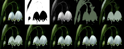
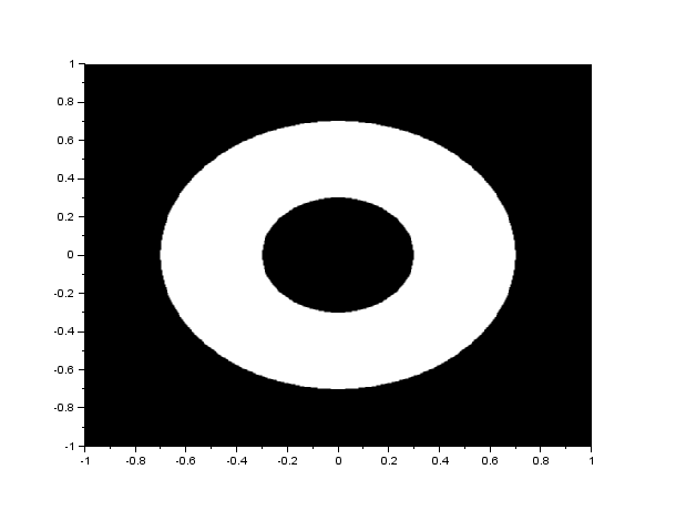
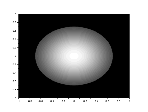
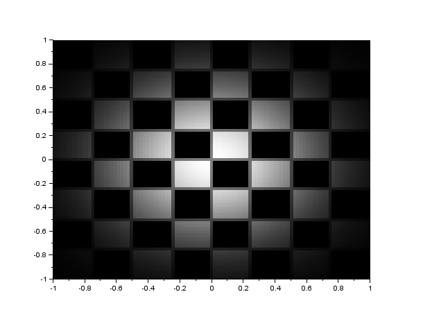
(A) True color (256 colors). (B) Binary. (C) Grayscale. (D) Indexed image, 2-colors. (E) Indexed Image, 4-colors. (F)Indexed image, 8-colors. (G) Indexed Image, 16 colors. (H) Indexed Image, 32 – colors. (I) Indexed Image, 64-colors. (J) Indexed image, 128-colors

The figure above shows a single image in 10 different types. We have the true color in 256 bit, black and white, grayscale and indexed images from 2-color to 128 color. In the hard-disk, the true color is 29 KB. The binary is considerably smaller in size, only about 21KB. The grayscale is 25KB. Now, it is worth noting that the indexed image is bigger than the true color image. (D-J is 30KB, 30KB, 32KB, 32KB, 31KB, 30KB, 29KB, respectively). We can see that indexing the image in 128 colors does not change the quality of the image, at least to a human observer. Though grayscale and binary has smaller file size, the smaller file size cannot compensate for the information lost. There are images in which the color is not important, but for this image, for the observer to appreciate the flower, full color, or at least indexing it at 128 color, is needed.

There are two types of image file format, classified according to how the images are formed. One is the raster images, which are composed of pixels and the vector images, which is composed of many tiny lines and curves called paths. [1] Let’s talk about them one by one. There are a lot of file extensions for the two types of images. I will only discuss the famous.

1. Vector images

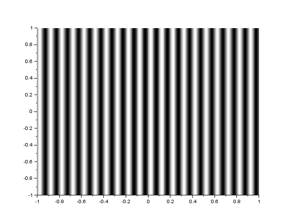
Vector images are images that are created using paths, in contrast to raster images which are made up of a grid of pixels. Thus, the images can be called as wireframe type images. These type of images must be created using specific computer softwares, since each path in the image has its own properties such as node positions, node locations, line lengths and curves. Vector images are very mathematical in nature, as to create these paths. [1,2] Since these images are not pixelated, vector graphics do not lose any quality if scaled into a larger size. This makes it ideal for logos, whose scale should be flexible.

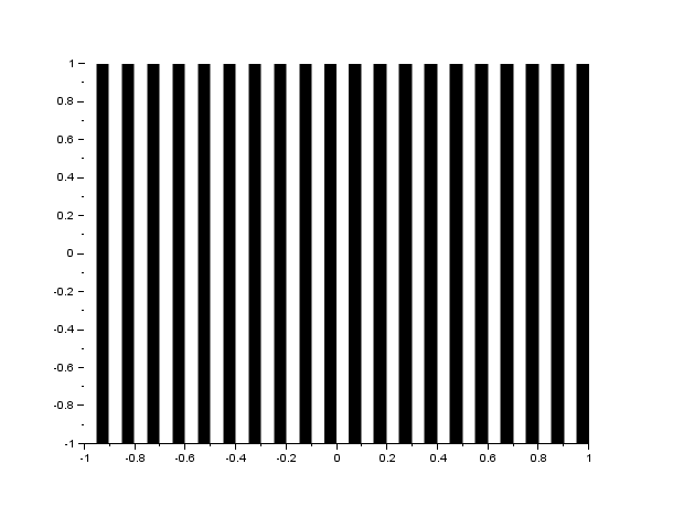
an example of a vector image

Vector file formats were the first kind of images that were used when the need to display output in devices came. The first display devices such as the CRT were similar to oscilloscopes, capable of producing and displaying geometrical shapes. When the need to store these images arose, the images were stored in a certain fashion. First, an image was subdivided into its simplest elements, meaning the paths. Then the image was produced, drawing each of its elements in the specified order. Lastly, data was exported as a list of drawing operations and the mathematical descriptions of the elements (size, shape, position) were written into the storage device in the order in which they are displayed. [3]

Some file types are shown below:

CGM (Computer Graphics Metafile)

• created by committees working under the International Standards Organization and the American Standards National Institute. It was designed as a common format for the platform independent interchange of bitmap and vector data, and used in conjunction with many different input and output devices. CGM sometimes incorporates extensions for bitmap images.[4]

• A very feature-rich format which attempts to provide the needs in many fields such as graphic arts, technical illustration, cartography, visualization, electronic publishing and others.

Gerber File Format

•  A standard electronics industry file format, often used in PCB manufacturing. The contents is in ASCII text. The contents are commands for a machine called photoplotter, which creates the picture on a photographic film by precise control of light.

There are other file types, often times extensions of files used by certain softwares such as the following:

AI (Adobe Illustrator), CDR(CorelDraw), HVIF(Haiku Vector Icon Format), ODG(OpenDocumentGraphics) and others.

2. Raster Images

Raster Images are images that are composed of tiny dots in a grid. All images I have displayed earlier (except for the example in vector) are raster images. The information of the picture are contained in each of the dots, and the information that is stored is only the color information. In contrast to vector images, no information about any line, angle or any mathematical shape is stored. Unlike vector images, the quality of raster images depend on the resolution; meaning the scaling is limited. If a raster image is scaled down, some pixel information have to be thrown away. and when a raster image is to be scaled up, to prevent loss of resolution, new pixels must be generated, of which the information it contains must depend on its neighboring pixels using a process called interpolation. There many techniques on resizing a raster image and compromising only a little bit of quality, but we will not delve on that here. 🙂

I will discuss some famous raster file extensions.

1. Bitmap (.BMP, .DIB)

• The bitmap as a raster file type image was created by microsoft and was first integrated into the Windows 3.0 os. This is due to the fact that BMP files were highly dependent on the graphics of the hardware used. The DIB supported only up to 16-bit of information per pixel then. (sorry i have no example. wordpress does not allow bmp. they’re not pro-microsoft, I guess. haha)

2. Joint Photographic Experts Group (.JPEG, JPG)

• JPEG is a method of lossy compression. It was a standard that was created by the group bearing the same initials in 1986, and since then have been adding more standards. The compression algorithm is a discrete cosine transform, converting the spatial information into frequency information then storing it. Since the transform is discrete, the resulting coefficients are quantized. In this compression scheme, the high frequency values are disregarded. This types of images are not for scientific use, nor for activities requiring high information. It is solely for human vision, since the omission of high frequency terms are not sensed by the eye. For examples, look at images in the web.

3. Graphics Interchange Format (GIF)

• GIF images employ a lossless compression format called the Lempel-Ziv-Welch lossless compression technique and was introduced to the world in 1987 by CompuServe. This was to provide a color format for file downloading areas of CompuServe. However, in 1995, the compression technique was patented by Unisys. This and the fact the GIF images are limited by the 256 color scheme made it undesirable. (http://en.wikipedia.org/wiki/Graphics_Interchange_Format)

4. Portable Network Graphics (PNG)

• The PNG is a lossless compression format that was desired as a replacement for the GIF. This is because the algorithm for the GIF was patented, and some limitations which rendered the GIF undesirable. Since the PNG employs a lossless compression format, it is often used in the scientific community.

Other Raster File Formats are the TIFF, IMG, DEEP, and others

The last part of the activity is to explore some SciLab syntax. Those are the following:

im = imread(‘imagefile’)// reads the image and name’s it as im

imshow(im)//shows image im

bw = im2bw(im, thresh)// converts im into a black and white image with respect to some threshold and then stores it as bw

histplot(numberofbins, array)// creates a histogram with number of bins.

imwrite(‘file’)// writes an image

imfinfo(‘file’, format)// returns information about the image file

 

The author would like to give himself a credit of 10/10. He would like to thank the ones who helped him: Hannah, and Abby. All of the images used are from the web.

sources:

fanpop.com
a1128.g.akamai.net
http://en.wikipedia.org/wiki/Dots_per_inch
http://www.dpreview.com/
http://www.laesieworks.com/digicom/compression.html
http://www.picturecorrect.com/tips/what-is-an-f-stop/

Using Exposure Bias To Improve Picture Detail

http://www.howstuffworks.com/what-is-iso-speed.htm

http://www.pcmag.com/article2/0,2817,1159326,00.asp
http://en.wikipedia.org/wiki/Graphics_Interchange_Format
1. Cousins, C. “Vector vs. Raster: What do I use?”. Design Shack. 6th Jun 2012. Accessed on 18 Jun 2013. Retrieved from http://designshack.net/articles/layouts/vector-vs-raster-what-do-i-use/
2. Faiza (username). “Basics, Difference Between Pixel and Vector-based Graphics”. Webdesigner. 13 Mar 2011. Accessed on 18 Jun 2013. Retrieved from http://www.1stwebdesigner.com/design/pixel-vector-graphics-difference/
3. Murray, James and vanRyper, Williams. Encyclopedia of File formats 2nd ed. Sebastopol: O’Reilly 1996. Print. Retrieved from http://netghost.narod.ru/gff/graphics/book/ch04_02.htm
4. Fileformat. “CGM File Format Summary”. Accessed on 18 Jun 2013. Retrieved from http://www.fileformat.info/format/cgm/egff.htm

 

Learning Scilab

In our Applied Physics 186 activity, we were told to tinker with Scilab programming language. It is a bit similar to Matlab, the language im familiar with. We used scilab to create some patterns and images, and yeah, it was fun.

For starters, we created a plot of a sine wave. The code was already given to us:

The code was pretty straightforward:

t = [0:0.05:100];
y = sin(t);
plot(t,y);

another code which was given to us was the code to create an image of a circular aperture. well, it was just a circle though, and to create it, some boolean was needed.

 

 

nx = 100; ny = 100; //defines the number of
elements along x and y
x = linspace(-1,1,nx); //defines the range
y = linspace(-1,1,ny);
[X,Y] = ndgrid(x,y); //creates two 2-D arrays of x
and y coordinates
r= sqrt(X.^2 + Y.^2); //note element-per-element
squaring of X and Y
A = zeros (nx,ny);
A (find(r<0.7) ) = 1;
f = scf();
grayplot(x,y,A);
f.color_map = graycolormap(32);

 

We were then instructed to create some patterns, as well as other shapes that we can create, as shown below (The codes are found in the last part of the post):

1. A centered square

2. Corrugated roof (sinusoid)

3. Grating along the x-direction:

4. Annulus

5. Circular aperture with graded transparency

I also created some other patterns:

A graded x_y grating:

An x grating with a beat frequency:

And an x-y grating with a beat frequency:

I also created other stuffs with the Fast Fourier transform, but that would have to wait. 🙂

I would like to thank Hannah Villanueva and Abby Jayin for the help of some of the codes. I would like to give myself a grade of 11/10 since I was able to create other patterns, aside from the patterns that were required.

codes:

centered square:

x = linspace(-1,1,100);
y = linspace(-1,1,100);
[X,Y] = ndgrid(x,y);
A = zeros(100,100);
A(find(abs(X)<0.7 & abs(Y)<0.7)) = 1;
f = scf();
grayplot(x,y,A);
f.color_map = graycolormap(32);

Corrugated roof:

x = linspace(-1,1,500);
y = linspace(-1,1,500);
[X,Y] = ndgrid(x,y);
x_sin = sin(2*%pi*X*10);
f = scf();
grayplot(x,y,x_sin);
f.color_map = graycolormap(32);

x-grating

x = linspace(-1,1,500);
y = linspace(-1,1,500);
[X,Y] = ndgrid(x,y);
x_sin = sin(2*%pi*X.*10);
A = zeros(500,500);
A(find(x_sin>0)) = 1;
f = scf();
grayplot(x,y,A);
f.color_map = graycolormap(32);

Annulus:

nx = 500; ny = 500;
x = linspace(-1,1,nx);
y = linspace(-1,1,ny);
[X,Y] = ndgrid(x,y);
r = sqrt(X.^2 + Y.^2);
A = zeros(nx,ny);
A_2 = zeros(nx,ny);
A(find(r<.7)) = 1;
A_2(find(r<0.3)) = 1;
ann = A – A_2;
f = scf();
grayplot(x,y,ann);
f.color_map = graycolormap(32);

Circular aperture with graded transparency:

nx = 500; ny = 500;
x = linspace(-1,1,nx);
y = linspace(-1,1,ny);
[X,Y] = ndgrid(x,y);
r = sqrt(X.^2 + Y.^2);
gauss = exp((-r.^2)/0.4)
A = zeros(nx,ny);
A(find(r<.7)) = 1;
gauss_circ = gauss.*A;
f = scf();
grayplot(x,y,gauss_circ);
f.color_map = graycolormap(32);

data reacquisition

What we did in class is that we scanned a hand-drawn plot from an old thesis[1], and try to recreate the plot by obtaining the pixel values. The aim of the activity is to be able to recreate the plot.

The image was scanned, and then opened in paint. Using the tick marks that can be found in the image, I obtained an equation that relates the pixel values to the real-world data from which the graph stemmed from. The x and the y axis had different relation equation given by the following:

f(x) = 5.02E-5*x + 1.15E-5

f(y) = 1.43E-5*y -6.10E-5

where f(x) and f(y) are the real world numbers and x and y are the distances from the origin of the graph in pixels. The y coordinate of the pixel posed a little problem since the values for y pixels go downward. The remedy is just to subtract the current pixel value from the value of the origin to find the distance in pixels.

Points along the curvature of the plot are then tabulated. Many plot points are obtained so that the resulting graph would be much more accurate to the real graph. I did both of the curves, the dashed and the continuous one, as seen from the image below.

The yellow and red dots are the graph that i obtained after getting the pixel values and converting them into real world values. It can be observed that some discrepancy exists. this is due to the fact that the scanned image is slightly tilted. I have not put a correcting factor on this because there is not enough time left.

I would like to give myself 11 total points, since I was able to overlay the graph that i obtained to the original one.

[1] Domingo, Zenaida (1980) Computer simulation of the focusing properties of selected solar concentrations, M.S. Thesis. UP Dilimanb