In our Applied Physics 186 activity, we were told to tinker with Scilab programming language. It is a bit similar to Matlab, the language im familiar with. We used scilab to create some patterns and images, and yeah, it was fun.
For starters, we created a plot of a sine wave. The code was already given to us:
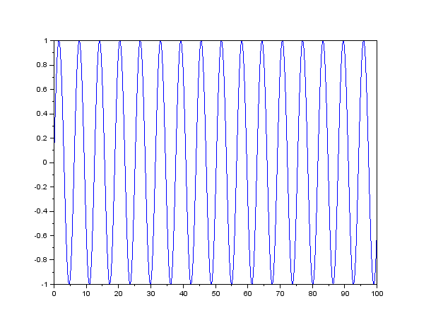
The code was pretty straightforward:
t = [0:0.05:100];
y = sin(t);
plot(t,y);
another code which was given to us was the code to create an image of a circular aperture. well, it was just a circle though, and to create it, some boolean was needed.

nx = 100; ny = 100; //defines the number of
elements along x and y
x = linspace(-1,1,nx); //defines the range
y = linspace(-1,1,ny);
[X,Y] = ndgrid(x,y); //creates two 2-D arrays of x
and y coordinates
r= sqrt(X.^2 + Y.^2); //note element-per-element
squaring of X and Y
A = zeros (nx,ny);
A (find(r<0.7) ) = 1;
f = scf();
grayplot(x,y,A);
f.color_map = graycolormap(32);
We were then instructed to create some patterns, as well as other shapes that we can create, as shown below (The codes are found in the last part of the post):
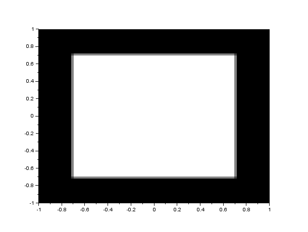
1. A centered square
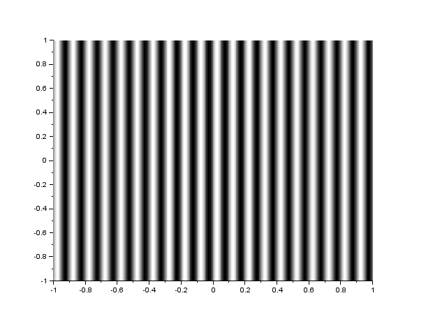
2. Corrugated roof (sinusoid)
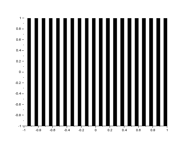
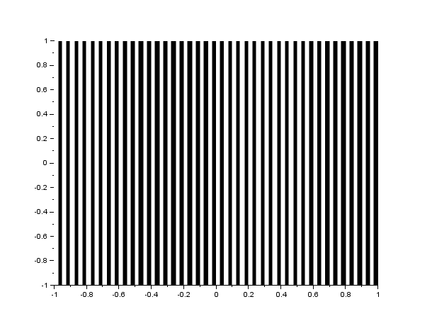
3. Grating along the x-direction:
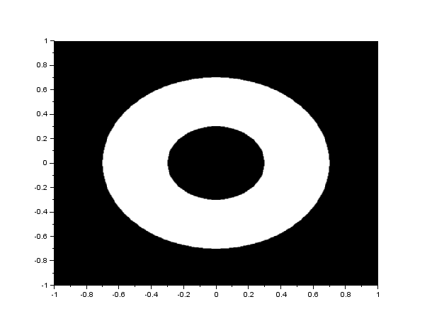
4. Annulus
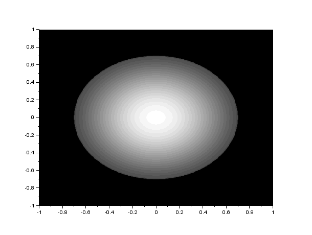
5. Circular aperture with graded transparency
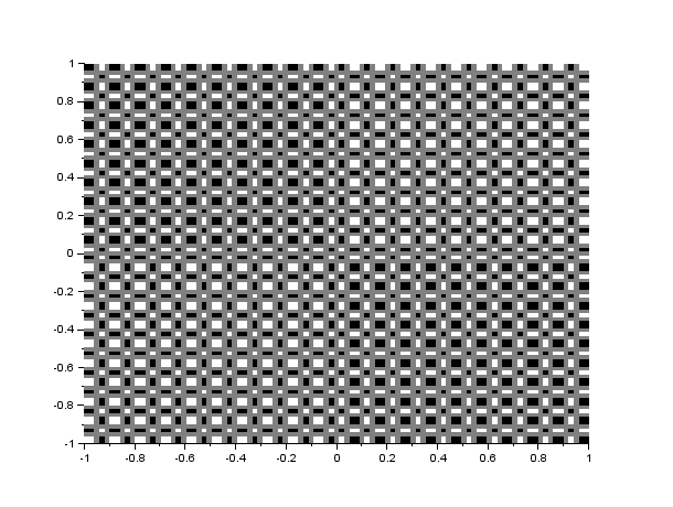
I also created some other patterns:
A graded x_y grating:
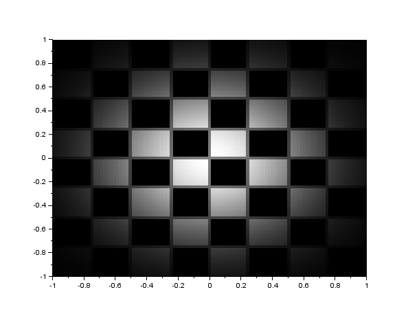
An x grating with a beat frequency:
And an x-y grating with a beat frequency:
I also created other stuffs with the Fast Fourier transform, but that would have to wait. 🙂
I would like to thank Hannah Villanueva and Abby Jayin for the help of some of the codes. I would like to give myself a grade of 11/10 since I was able to create other patterns, aside from the patterns that were required.
codes:
centered square:
x = linspace(-1,1,100);
y = linspace(-1,1,100);
[X,Y] = ndgrid(x,y);
A = zeros(100,100);
A(find(abs(X)<0.7 & abs(Y)<0.7)) = 1;
f = scf();
grayplot(x,y,A);
f.color_map = graycolormap(32);
Corrugated roof:
x = linspace(-1,1,500);
y = linspace(-1,1,500);
[X,Y] = ndgrid(x,y);
x_sin = sin(2*%pi*X*10);
f = scf();
grayplot(x,y,x_sin);
f.color_map = graycolormap(32);
x-grating
x = linspace(-1,1,500);
y = linspace(-1,1,500);
[X,Y] = ndgrid(x,y);
x_sin = sin(2*%pi*X.*10);
A = zeros(500,500);
A(find(x_sin>0)) = 1;
f = scf();
grayplot(x,y,A);
f.color_map = graycolormap(32);
Annulus:
nx = 500; ny = 500;
x = linspace(-1,1,nx);
y = linspace(-1,1,ny);
[X,Y] = ndgrid(x,y);
r = sqrt(X.^2 + Y.^2);
A = zeros(nx,ny);
A_2 = zeros(nx,ny);
A(find(r<.7)) = 1;
A_2(find(r<0.3)) = 1;
ann = A – A_2;
f = scf();
grayplot(x,y,ann);
f.color_map = graycolormap(32);
Circular aperture with graded transparency:
nx = 500; ny = 500;
x = linspace(-1,1,nx);
y = linspace(-1,1,ny);
[X,Y] = ndgrid(x,y);
r = sqrt(X.^2 + Y.^2);
gauss = exp((-r.^2)/0.4)
A = zeros(nx,ny);
A(find(r<.7)) = 1;
gauss_circ = gauss.*A;
f = scf();
grayplot(x,y,gauss_circ);
f.color_map = graycolormap(32);
